by Fred Steinhauser, OMICRON electronics GmbH, Austria
The time performance of protection and automation systems was always a crucial topic. One very important aspect of the performance of protection systems was testing the trip times in the first place. Besides the speed of the protection algorithms itself, other contributors as debouncing filters and contact delays were well known. With the proliferation of IEC 61850, the communication services GOOSE and Sampled Values are applied for mission critical real-time messaging. The time delays induced by the communication components, which can be the processing times in the communication stacks in the protection and automation devices and the transmission times in the communication networks, are now affecting the performance. Thus, it is desirable or even necessary to know about this timing performance. This must be regarded when designing such a system and finally it has to be verified by measurements.
What is latency?
As it has become good practice, let us first check what Wikipedia says:
Latency is a time interval between the stimulation and response, or, from a more general point of view, a time delay between the cause and the effect of some physical change in the system being observed.
Not everything written in Wikipedia is unquestionably reliable, but this general definition actually describes very well also our case in the digital grid. The stimulus may be a data change to be communicated and the response may be an action taken at the receiving end. If we really wanted to bring in a physical change this could be a disconnector switch changing position or a power system fault.
We will use the term latency for the entire overall time delay in the following and state that it is made up from several contributing times, that we will call delays.
Example: the round-trip test
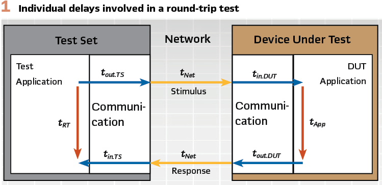
This test, also called “ping-pong test,” is proposed in the GOOSE performance test procedures published by the UCA International User Group. Other than most of the tests explained below, it does not at all focus on network latencies, but it serves as an example of how distinct delays can be extracted from a latency measurement. This test is performed to determine the GOOSE processing delay of the IED under test from a latency measurement, in this case the round-trip time. (Figure 1).
Several preconditions must be met to make a useful evaluation. The network delay must be negligible, the test set delay and the application delay must be known, and symmetry of the input/output delays must apply. Of course, the measurement is repeated many times to allow sensible statistical evaluation. So, the measurement of the latency may not be the actual goal of the test, but a mean to deduct other results.
The test laid out above is one that can be performed with a finished product without special instrumentation for the measurement within the product.
This was the reason that it was included in that form in the GOOSE performance test specifications. It is also a test where the measurements are entirely done with network messages for the stimulus and the response. In a development lab, such tests would be done with additional test pins to get access to intermediate events to isolate the individual delays more specifically. Likewise, latency measurements in Smart Grids may not be only done with network messages, but also with hard wired signals such a breaker auxiliary contacts.
Communication Latencies
Tests assessing the timing of binary I/Os, be it an attribute in a GOOSE message or a physical contact of an IED, are performed since the early 2000s with advanced protection test sets. Such devices, which process signals from both worlds, networked and classical, are also called “hybrid.”
In the course of so-called end-to-end protection tests, such tests were also performed in a distributed scenario. As this processing of binary I/Os can be called a long established procedure, it shall not be in the focus of this article.
In the rest of this treatise, the subject will be communication latency measurements from captured Ethernet packets. Such packets must be captured in at least two locations. An algorithm will then evaluate the differences from the time stamps of the same packet occurring at the different locations. As a large number of packets is typically involved in such a measurement, statistics can be derived.
Matching the occurrences of an individual packet at the different locations is easy when all of them are captured in the same local network (within the same broadcast domain), since the Ethernet packets are not modified within this scope. GOOSE and Sampled Values are typical examples for network traffic used for such measurements. But when the tests are performed with IP packets via routed networks, the modification of certain fields in the IP packets need to be regarded.
It’s all about timing
To measure latencies, events must be acquired with sufficiently accurate time stamps from which the results will be calculated. To assure this accurate time stamping, the time synchronization of the measurement equipment is crucial. Depending on the test case, different requirements exist.
As a latency to be measured is a time difference, the absolute time maintained by the measurement system does not matter in the first place, since it cancels out when the difference of time stamps is calculated. If the measurement can be made with both the stimulus and the response captured by the same device, the absolute time maintained in the internal clock of the device is irrelevant for the latency measurement.
Typically, high precision oscillators with an error of only a few parts per million are used to drive the clock in such devices. The error for the time stamping of the captured Ethernet packets can be well below 100 ns. Thus, the latencies determined that way are very accurate.
As soon as two or more acquisition devices are used, they need to be time synchronized in some way. In a local setup, for instance in a factory acceptance test (FAT), multiple acquisition devices may be synchronized over a local network. It is becoming more and more common to use the precision time protocol (PTP, IEEE 1588) for time synchronization in power utility applications.
When this time protocol is anyway used to synchronize the protection and control devices in the power utility communication network, the measurement devices can also synchronize to the same clock. But even if PTP is not yet used in the system under test, a small test control and time synchronization network connecting the measurement devices is often a convenient way to synchronize such a local measurement setup. For testing, a time source can be used even if it is not globally synchronized to “the rest of the world,” as long the devices involved in the test setup are properly synchronized in relation to each other.
There are also options that a test set may work as a time master for other test devices, synchronizing all of them to a common time reference.
When the system to be tested spans over larger distances than in a FAT, different solutions must be employed. Already in a commissioning situation, distances in a large substation can easily span over hundreds of meters. While such distances could still be bridged with long network cables to bring the traffic to a single capture device, this may not be desirable anymore, although this still seems to be much more feasible for network signals than for classical binary I/Os. For wiring classical signals to the measurement devices, the devices need to be close to the access points. Also, the number of signals to be captured may exceed the capacity of a single capture device in such setups.
This is then an application for multiple time synchronized capturing devices, a so-called distributed measurement scenario. When the network infrastructure in the substation does not yet provide PTP for time synchronizing the measurement devices, other time sources need to be considered.
The most prominent option is obtaining the time from Global Navigation Satellite Systems (GNSS), as there are GPS, GLONASS, Beidou, and Galileo. Each capture device will then have its own GNSS receiver assigned, synchronizing each device to a global time reference.
This distributed measurement scenario applies even more when stimuli and responses are to be collected from access points located far from each other, as for example from different substations. Either PTP (fed from a global time source) is available in these substations, or the scenario with individual GNSS receivers for each capturing device apples again. Also, a mixed time synchronization setup will work, by using dedicated GNSS receivers only in places where PTP is not available.
The accuracy with using GNSS is perfectly adequate for the intended purpose, time errors below 1 µs are easily achievable.
Centralized Measurement Setup
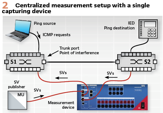
A very minimalistic example for a local, centralized measurement setup with a single capture device only processing Sampled Values is shown in Figure 2.
The capture device used its free running internal clock with no synchronization to a global time reference. The latencies were calculated as the difference of the time stamps from packets before entering the network and the same packets reappearing at the opposite end of the network.
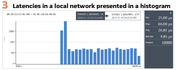
This setup was chosen to evaluate the influence of network load on the propagation of Sampled Values in an Ethernet network. The network load was created by flooding the network with Ping requests with different parameters. The latencies for thousands of packets were collected and presented in a histogram in Figure 3.
In this centralized case with only one capture device involved, the control of the measurement system is trivial, as no coordination with other devices is required.
Distributed Measurement Setup
The various flavors of distributed measurement setups have been already indicated above in the chapter about the different options for time synchronization.
In a distributed scenario within a substation, certain simplifications will most likely apply. Typically, a local area network exists that connects all the IEDs.
The measurement devices can be also connected to this network, providing straight forward access to the capture devices and simplifying the control of the measurement system. Possibly, the local network also provides PTP, which also serves the time synchronization of the capture devices.
This case is relatively easy to master and will not be elaborated any further.
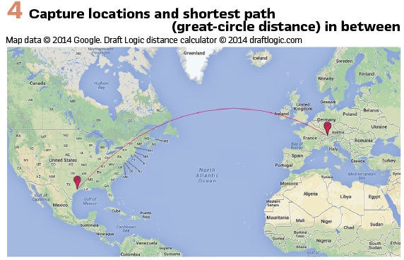
To explore the extremes and as a proof of concept, a latency measurement was performed between two locations in two different continents. It is unlikely that time critical data for protection, automation and control will be exchanged over such a distance, but it shows the orders of magnitudes that can be expected for the latencies. Figure 4 illustrates the locations of the two involved sites in Austria and in Texas.
Of course, such wide area network connections involve routing, which means that several convenient features that are available in local networks, as for finding devices, do not work anymore. The network masks and gateways in the sub-networks and the IP addresses of the involved devices need to be known and properly set within the communicating devices to ensure connectivity for controlling the measurement system.
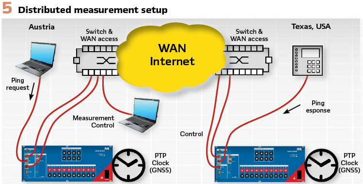
The test setup involved two capturing devices, both individually time synchronized with a dedicated GNSS receiver. The control of both devices was performed via the internet from one side only. (see Figure 5).
The test was performed with ICMP packets (Ping requests and responses). The network links to the devices exchanging the Ping packets were tapped by the capture devices.
The requests were sent from Austria to Texas, the responses went back from Texas to Austria. Each packet type delivered the data for one of the directions. Figure shows the network latencies individually in each direction.
It must be pointed out that this measurement delivers the individual latencies for each direction, which adds significant value. This is an essential progress compared to measuring the round-trip times with the Ping command alone. The round-trip time includes the (typically unknown) reaction time of the device answering the requests before sending back the response. And even if the reaction time could be deducted, the remainder is the sum of the latencies in both directions, not delivering any clue if they are about equal or if they differ and for how much.
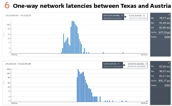
The measured latencies were in the range of 80 ms to 100 ms. To zoom in and show the distribution in more detail, the graphs are biased at 70 ms and the distributions are much narrower than the figure suggests. Most of the latencies lie close to the average values of 82 ms or 84 ms respectively. There are only very few outliers, none of them exceeding 100 ms. The standard deviations are less than one percent of the mean values in both directions.
The great-circle distance between the two locations is about 8654 km. As the communication links will not be laid out along the great-circle, let us round this up to 12 000 km. With the typical value for the speed of the wave propagation on electrical wires or in optical fibers (about 2/3 of the speed of light in the vacuum), the propagation time in the media for this distance equals about 60 ms. This leaves about 20 ms to 40 ms for the processing and forwarding of the packets in the involved communication equipment.
Finding out more
The following example comes from a measurement taken between two locations in Central Europe, about 275 km apart (great-circle distance). Such a distance seems practical for distributed protection and automation applications.
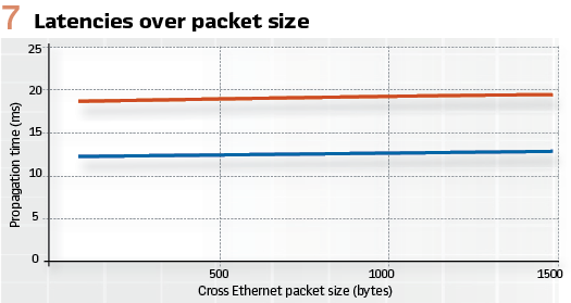
This test was conducted with the aim to conclude more about the properties of the communication link than just the latencies alone. To do so, the latency measurements were made with different packet sizes, which is shown in Figure 7.
The link is obviously not symmetrical, the latency in one direction is about 12 ms, while it is about 19 ms in the other direction. But it is also visible that there is a dependency of the latency from the packet size. The slope of the two lines is 500 ns/byte. This delivers an effective link speed of 16 Mbit/s. This conclusion was possible from the measured latencies even though we have no actual data of the wide area links.
Again, it must be assumed that the actual links are not laid out along the great-circle through the two locations, so the path length may be up to to 400 km. With the speed of light in the communication media, we can estimate the propagation time in the media to about 2 ms.
The rest of the time (about 10 ms and 17 ms) is used for encrypting the data in the virtual private network and for forwarding the packets in the network components. This also explains the asymmetry, because different equipment with different performance was used on the two ends for the encryption/decryption of the data. Thus, the results obtained from such measurements give clues for improvements in the communication infrastructure if required.
Conclusions
Knowing about the latencies in power utility communication networks is crucial. Measuring them provides information about the performance of the communication and finally the performance of the protection, automation and control system.
The measurement results mentioned above give hints on the order of magnitude of the latencies to be expected in different scenarios. In a local area network, a few dozens of microseconds (at a link speed of 100 Mbit/s) are typical. And when going to higher link speeds, the latencies will shrink accordingly.
In the shown distributed scenario, which is extreme since it spans over almost one quarter of the earth’s circumference, the latencies remained well below 100 ms.
For realistic wide area applications with dedicated power utility communication networks, a few dozens of milliseconds may be an upper limit.
By repeating the measurements with varied parameters (such as different packet sizes), further conclusions about the nature of an otherwise hidden communication link can be made.
With the latest advancements of measurement tools, the measurement of network latencies has come within the reach of the power utility engineers.
There are several options for proper time synchronization of the measurement system and the centralized control of also remote capture devices provides ease of use for the performance of distributed latency measurements.
Biography
Fred Steinhauser obtained a diploma in Electrical Engineering from the Vienna University of Technology, and a Dr. of Technical Sciences in 1991. He joined OMICRON and worked on several aspects of testing power system protection. Since 2000 he worked as a product manager with a focus on power utility communication. Since 2014 he has been active within the Power Utility Communication business of OMICRON, focusing on Digital Substations and serving as an IEC 61850 expert. Fred is a member of WG10 in the TC57 of the IEC and contributes to IEC 61850. He is one of the main authors of the UCA Implementation Guideline for Sampled Values (9-2LE). Within TC95, he contributes to IEC 61850 related topics. As a member of CIGRÉ he is active within the scope of SC D2 and SC B5. He to the synchrophasor standards IEEE C37.118.1 and IEEE C37.118.2.