by Fred Steinhauser and Florian Fischer, OMICRON electronics, Austria, and Walter Sattinger, Swissgrid, Switzerland
Phasors are indispensable for the mathematical mastering of electrotechnical phenomena. The mathematical operations for complex numbers apply and with impedances also given in such a complex form, further calculations are possible, as well as calculating the “complex powers” from the current and voltage phasors.
From Phasors to Synchrophasors
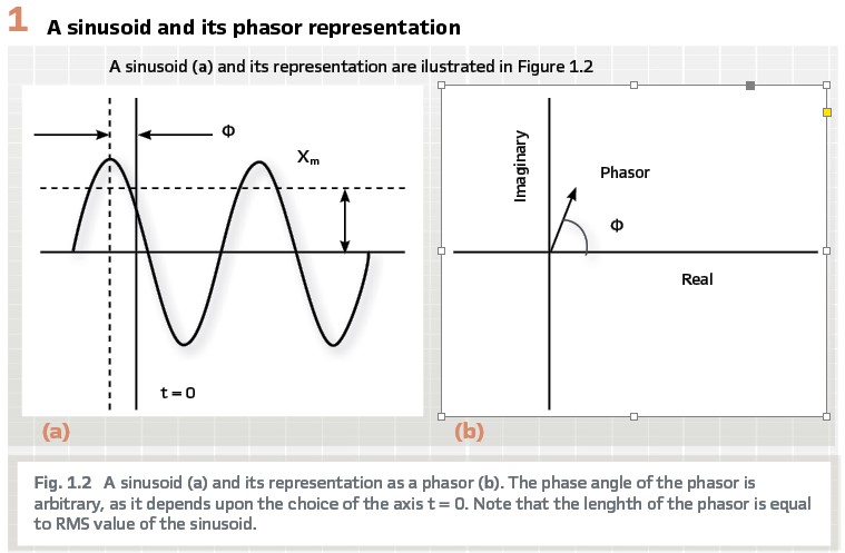
The definition of a phasor given above says about the phase: it is arbitrary, depending on the context.
For synchrophasors, the context is defined by a reference sinusoid, whose frequency is the nominal frequency of the electrical power system (in the following just called “nominal frequency,”) and which has its positive maximum at the top of the UTC second. In that sense, it could be called the reference cosinusoid. All phases of synchrophasors are specified in relation to this reference cosinusoid.
To reiterate the synchrophasor definition, here comes a key sentence from the introduction chapter of IEEE C37.118.1, the standard that helped to make synchrophasors popular: “A synchrophasor is a phasor value obtained from voltage or current waveforms and precisely referenced to a common time base.”
Not just having the magnitude measurements, but also the phase information of the electrical quantities in the power network, referred to the same reference signal, no matter where the measurements come from, adds an entirely new quality to the data. Calculations, analyses, and finally conclusions are now possible which could not be done without the phase information.
The sufficiently precise common time reference is crucial, but this was difficult to establish over wide areas for a long time. In this sense, the availability of GPS since the mid-1990s was an enabler for the implementation of phasor measurement devices, although this matter has become more complex today.
And as these phasor measurements must be forwarded to a central instance that collects and processes all these data, the availability of suited communication channels and networks was also such an enabler. This has rapidly evolved since the 1990s as well.

The synchrophasor standard employs clear and precise terminology and refrains from quirky definitions of a phasor like “a rotating vector” or so, as phasors and vectors are something different and have little in common (see PACW Magazine December 2018, p. 17: “Phasors are not vectors.”) The term “vector” appears only in the term “Total Vector Error” (TVE), where it could be argued why this was not named “Total Phasor Error.” Note that the term “amplitude” also has no place here, since the magnitude of a phasor is the RMS value of the voltage or current.
About PMUs
The synchrophasors are delivered by measurement devices called Phasor Measurement Units (PMUs).
The synchrophasor standard IEEE C37.118.1, again in the introduction, describes such devices this way: “The PMU extracts the parameters magnitude, phase angle, frequency, and ROCOF from the signals appearing at its input terminals.” (ROCOF stands for “rate of change of frequency”, the first derivative of the frequency).
The standard IEEE C37.118 was superseded by IEEE/IEC 60255-118 which is now the normative document for all things related to synchrophasors and PMUs. In the following, it will be referenced simply as “the standard.”
The standard gives a reference implementation in annex D as an example. In this case, it is a synchronous demodulator, but other concepts for measuring synchrophasors are well possible and in use.
In any case, the voltages and currents from the power network are digitized, delivering the so-called samples. The phasor calculations are performed by a computer algorithm processing these samples. The synchrophasors are then forwarded via a communication interface, typically to a phasor data concentrator (PDC), which aggregates the phasor data and provides them to an application.
Sampling and reporting rates
It might be worthwhile to recall the difference between two terms occurring in this context: the sampling rate (the frequency for sampling the voltages and currents at the input of the PMU), and the reporting rate (how often calculated phasor data are sent out by the PMU).
In a well-designed system, any data rate is in a sensible relationship to the dynamics of the system. For sampling values, this is commonly known as the sampling theorem. It puts the frequencies occurring in the system into a relationship to the Nyquist frequency.
As the phasor calculation focuses on the fundamental component which is expected to be close to the nominal frequency, decent sampling frequencies are sufficient. Given the restrictions for implementing suited anti-aliasing filters, a phasor calculation can be well done with a sampling rate of about 16 samples per cycle. The examples given in annex D of the standard support this.
Without going into the differences between P class and M class PMUs, there is “… the need to include at least one cycle of the power system waveform …” for a sound phasor calculation (clause 6.7, note at table 10). Well, there are methods, e.g., used in protection algorithms, to estimate phasor properties from sub-cycle windows, but then this degenerates really towards an estimation and cannot be considered a measurement. The relationship between the input data length (window length) and the frequency response is comprehensively explained in annex D. The result is a low pass characteristic. For a so-called rectangular window (the input samples are not weighted) with the duration of one cycle (window length = 1/nominal frequency), the first zero of the frequency response is at the nominal frequency. Other windowing functions may change these relationships in some way but will not remove the fundamental fact that there is a time constant limiting the dynamic response of the phasor calculation. When the window length increases (as for M class PMUs), the bandwidth is further decreased, which means that the PMU reacts slower on changes of the input quantities. Bottom line, the phasor calculation itself introduces a relevant time constant into the measurement chain. Thus, reporting rates such as twice or quadruple the mains frequency may be called not economical in the least. More is not better. Pushing the reporting rate beyond one per cycle produces more data, but without delivering more information.
On a large scale, the power system itself is even more sluggish, essential changes of the overall system state do not take place within one cycle only. As a rule of thumb, reasonable state estimation of large power systems can be well done with a reporting rate of 10 phasors per second.
Accuracy and Total Vector Error
The accuracy requirements for PMUs are expressed as a permissible Total Vector Error (TVE). The TVE is made up of two components: the magnitude error and the phase error. Annex C.2 of the standard explains how the TVE is composed, also outlining that none of the components can take all of the margin for itself, there must be left some leeway for the error of the other component as well.
The understanding of the magnitude error is trivial. The phase error translates into a time error, ultimately leading to the permissible uncertainty of the time synchronization of the PMU.
Time Synchronization of PMUs
There are various myths surrounding the requirements for time synchronization of PMUs. Let us look at this starting at the 1 % TVE figure for PMUs as specified in the standard. Clause 4.6 of the standard gives the related time errors of about 27 µs (for a system frequency of 60 Hz) and 31 µs (50 Hz). Figure 2 shows the relationship between magnitude error, time error, and TVE for a system frequency of 60 Hz.
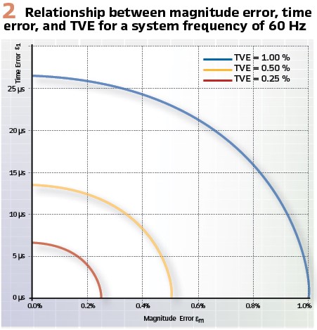
This diagram in Figure 2 is equivalent to Figures C.3 and C.4 in the standard, but not only exploits the symmetry in one component, it does this for both components, mapping the whole context into one quadrant and one single diagram. It shows, for example, that a PMU with a magnitude error of 0.4 % and a time error of 5 µs would stay within the limit for a TVE of 0.5 % given by the yellow arc.
The following considerations, which are mainly intended to point out the orders of magnitude we have to deal with, are based on an average “rule of thumb” value for the maximum time error of about 30 µs.
In clause 5.4.2 (Compliance verification), the standard states a desired TVE for calibration devices ten times smaller than 1 %, which is 0.1 %. It should be noted that IEEE C37.118 said that a calibration equipment must be four times better (i.e., have a TVE < 0,25 %) than the PMU to be calibrated. This is sufficient from a metrology point of view, just more demanding in terms of evaluation of the results than going with the larger margin of “ten times better.”
It is obvious that the required accuracy alone for the magnitude measurement is challenging. Since one error component must not take up all the margin alone, the magnitude error must be considerably less than 0.1% which exceeds the most demanding accuracy class 0.1 for metering. For the time synchronization, this would mean timing uncertainties lower than about 3 µs, which is still not overly challenging from the point of time synchronization. These 3 µs correspond to about 0.06° or 3.4 arc minutes.
To put this into perspective, IEC 61869-2 and –3 for CTs and VTs allow a phase error of 5 arc minutes (or 0.08°) for class 0.1 instrument transformers, which translates into a time error of about 4 µs. See Table 1.
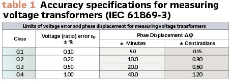
This means, for a measurement system, a TVE of 0.1% over the whole signal acquisition chain will be hardly achievable with today’s series produced devices, but the limiting factor would not be the time synchronization of the PMU. There may be mtrology grade equipment that can reach these specs, but this has no relevance for practical applications in the field.
For the time synchronization of merging units publishing Sampled Values according to IEC 61850-9-2 / IEC 61869-9, the aim is an uncertainty of the time synchronization below 1µs. This is backed by the requirements in the Precision Time Protocol (IEEE 1588) profiles as described in IEC 61850-9-3 and IEEE C37.238. Thus, the timing means for IEC 61850 Digital Substations are more than sufficient for time synchronizing PMUs as well. There are no timing accuracy requirements in the sub-microsecond range for PMUs.
Communications – transmitting the synchrophasors
Synchrophasors are mostly transmitted over larger distances, using so-called wide area networks (WANs). The method of choice is to use the internet protocol and the associated transport layer protocols.
Most implementations use the message format described already in the initial version of IEEE C37.118. On the transport layer, variants with TCP and UDP are in use.
A requirement to communicate synchrophasors “the IEC 61850 way” resulted in the development of IEC 61850-90-5. The periodic nature of synchrophasors matches the IEC 61850 Sampled Values. But as of 2009, when this work was started, there was only a mapping for Sampled Values on Ethernet layer 2 for the use in local area networks. This protocol was not equipped for routing through a WAN. Thus, a routable version of Sampled Values (R-SVs) was laid out in IEC 61850-90-5. In the same course, an equivalent mechanism was created for routable GOOSE messages (R-GOOSEs). Meanwhile, these routable variants of GOOSE and SV were included in IEC 61850-8-1 and IEC 61860-90-5 was deprecated. While the R-GOOSE is gaining popularity, the R-SVs are rarely used. R-GOOSE and R-SVs come with methods to ensure cyber security. Although routable, they are generally not transmitted over unprotected public communication networks, but over utility owned, protected networks, so that the application of additional cyber security measures is not necessary, thus saving efforts.
Communication latencies do not impair the quality of the synchrophasor data since each reported phasor value carries its precise time stamp. The PDC or application must wait until all data from all PMUs have arrived before aggregating or processing the data. This will delay the action until the last data for a certain point in time has arrived. But with today’s high performance communication networks, this delay will be insignificant in most cases. Only for fast acting wide area protection applications working with synchrophasors from P class PMUs, the latencies must be closely observed.
Testing PMUs
Annex C of the standard provides guidance for testing the metrics laid out and specified in chapter 5. Testing of PMUs is done in different contexts, to mention development, certification, and deployment.
During PMU development, accurate industrial grade signal sources provide test signals and mostly custom-made software controls the signal generation and evaluates the measured synchrophasors for an assessment. The efforts are driven high enough to be confident that the product will pass the certification.
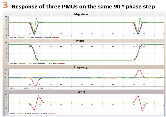
Figure 3 shows some results obtained by applying test signals to PMUs through a precise industrial 3-phase test set, controlled with a ready-made software.
PMU Certification is usually carried out at metrological institutes that have metrology grade PMU testing facilities. These test systems are custom built from high-precision components and are only produced in small quantities or are even unique.
At deployment, the accuracy of the PMU is not tested. There is no reason to assume that the certified product would not be in spec. There may be a need to verify the correct wiring of the input signals, the proper time synchronization, and the functioning of the communication to report the synchrophasor data. Routine testing of PMUs is not considered necessary as the devices are continuously in operation and in some way supervised, as a failure would become obvious through inconsistent measurements or even disrupted delivery of the data.
A sidenote on Harmonics
A significant portion of the PMU tests are about disturbed signals (not pure sinewaves), particularly containing harmonics. A PMU is by nature a narrow bandwidth device. The synchrophasors are the representations of the fundamental components of the quantities in the power system. The frequency of this fundamental component is assumed to be within a few Hertz (giving the actual value is complicated) around the nominal frequency of the power system. This is called an “in-band” signal and the synchrophasor measurement is to determine this “in-band” component. On the other hand, the synchrophasor measurement shall be as little as possible affected from signal components outside this frequency band (“out-of-band” components) such as harmonics. Thus, the job of a PMU is not to react on harmonics, but to suppress them as much as possible. Or in other words, the purpose of PMU tests with harmonics is to prove that the synchrophasor measurement is not impaired due to the presence of harmonics.

Modeling and Simulating WAMS Scenarios
To investigate the phenomena in electric power systems, observe the related effects at different measurement points, and to verify the assessment and reactions of a wide area monitoring system (WAMS), simulation of the system is a valuable option. This is the domain of Real Time Digital Simulators in which the power system is modeled in much detail. Depending on the sophistication of the model, the effects will be simulated close to reality. The only drawback of these large scale RTDS systems is that they can only be applied in the lab. Using them on site is not an option.
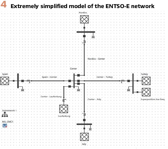
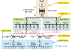
Figure 4 shows an extremely simplified model of the ENTSO-E Continental Europe power system, spanning from Spain to Turkey (west to east) and from the Nordic countries (Denmark, Poland, Baltics) to Italy (north to south) with a center assumed in the vicinity of Switzerland. It neglects any details, so the signals simulated from this model are by far not as realistic as from the RTDS system mentioned above. But it preserves the fundamental connections and the power flow between the distributed load and infeed areas of the system.
The relationships between the quantities in this simplistic power system will be consistently reflected in this model. On the east busbar, a second infeed is connected for introducing disturbances into the system. In this case, it superimposes a power fluctuation due to a pole slip with a duration of two seconds. Figure 5 shows how this power fluctuation appears at the western side.
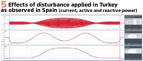
The phenomenon simulated in this example is exaggerated for obvious illustration, but by adjusting the parameters of the superposition infeed, the effects can be modeled adequately subtle.
Such simulations can be made with a simulation system that controls test devices deployed in arbitrary places to physically apply the simulated signals to devices under test. This way, the test signals can be applied to the deployed PMUs to test the overall WAMS. The test scope will include the operation of the PMUs, the communication of the synchrophasor data and the reaction of the WAMS application.

Verifying WAMS Functions
One typical inter-area oscillation occurred in the Continental European (CE) power system on Dec. 3rd, 2017, where the entire Italian peninsula oscillated against the rest of the CE power system (see Figure 6) as recorded by CE WAM systems. For about ten minutes frequency fluctuations of 300 mHz peak-to peak occurred in the Southern part of Italy, see Figure 7.
As main cause of the incident the following combination of impacting factors were identified:
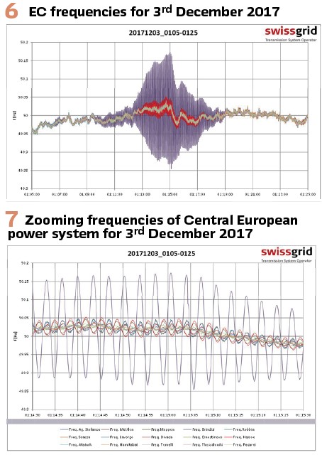
- Very low consumption – decrease of load contribution for damping
- High voltage phase angle difference between North and South of Italy
- Unavailability of some generators with good damping behavior
- High import in the Southern part of the CE power system
The prompt reaction of the Italian control room staff has saved the situation as they have performed an internal re-dispatch and disconnected a shunt reactor in the Southern part of Italy accordingly.
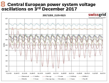
However, the resulting huge active power oscillation on the Northern Italian border have resulted in related significant voltage oscillations with peak values of up to +/- 2.5 kV on the 400 kV transmission layer, see Figure 8.
In fact, the presence of an Online WAM system in the Italian control room has led to a fast mitigation of the critical North-South inter-area mode in the CE power system as related countermeasures were already pre-prepared available.
Outro
Since the upcoming of the synchrophasors in the 1990s, the topic has evolved in an interesting way. The principles and basics were well described from the beginning. IEEE C37.118:2005 was already encompassing and solid and specified well what a PMU must deliver. The standard has been developed further, adding features, or defining them in more detail.
On top of the foundation provided by the availability of the synchrophasor data, the related applications have dynamically evolved over the past two decades. We now have tools to monitor the state of the electrical power grid that support keeping it stable and the lights on. Synchrophasors are “Big Data” and the options to make something useful out of this are again expanding with the hype around artificial intelligence. No matter how this stimulates our fantasy, what we have, and use based on synchrophasors is already indispensable.
Biographies:

Fred Steinhauser studied Electrical Engineering at the Vienna University of Technology, where he obtained his diploma in 1986 and received a Dr. of Technical Sciences in 1991. He joined OMICRON and worked on several aspects of testing power system protection. Since 2000 he worked as a product manager with a focus on power utility communication. Since 2014 he is active within the Power Utility Communication business of OMICRON, focusing on Digital Substations and serving as an IEC 61850 expert. Fred is a member of WG10 in the TC57 of the IEC and contributes to IEC 61850. He is one of the main authors of the UCA Implementation Guideline for Sampled Values (9-2LE). Within TC95, he contributes to IEC 61850 related topics. As a member of CIGRÉ he is active within the scope of SC D2 and SC B5. He also contributed to the synchrophasor standard IEEE C37.118.

Florian Fischer studied electrical engineering at the Friedrich-Alexander University Erlangen-Nuremberg (Germany). Since 2013, he has been working as a protection engineer for OMICRON Germany. He has been involved in creating automated test plans and developing and conducting trainings for OMICRON Academy. For many years, he supported customers on the topics around IEC 60255 standard testing, test automation and specifying test routines. Since 2022 he is the responsible Product Manager for the system-based testing solution RelaySimTest.

Walter Sattinger has a degree in Electrical Engineering and PhD from the University of Stuttgart, Germany. For eight years he was a Research Assistant at DIgSILENT company. Since 2003 he is a power system expert at ETRANS/Swissgrid on the interface between power system operation and power system planning. Today he is responsible for the operational/ technically interface to power plants operators, distribution systems operators, transmission system and foreign power systems operators.